Supervised Learning and Linear Models

Introduction

For the beginners of machine learning like me, the first concept is always the linear models of supervised learning. In this post, I will go through some basic terms of supervised learning and several useful linear models.

A quick overview of concepts covered in this post:

• Supervised Learning
  • Train and test datasets
  • Model & hypothesis & hypothesis space
  • Training process and prediction
  • Loss function and objective function
  • Model Utilities: Classification vs. regression
  • Model Fitting: Overfitting vs. underfitting
  • Model Fitting: Variance vs. bias trade-off
• Linear Model_1: Linear threshold units (LTUs) and Perceptron
• Linear Model_2: Logistic Regression
• Linear Model_3: Linear Discrimination Analysis (LDA)
• Model Optimization: Gradient Descent Algorithm

Supervised Learning

What is supervised learning?

Based on boring definition, supervised learning is a type of machine learning algorithm where the model learns to make predictions by being trained on a labeled dataset. In simple terms, the model knows the input data and the corresponding correct output, and the goal is to learn the mapping between the two. Other types of machine learning are unsupervised learning and reinforcement learning.

Here comes the first term: Train and test datasets

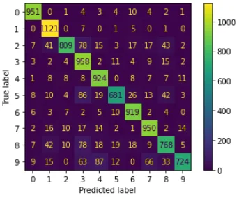
The training set is used to fit the parameters of the model, such as the weights in a neural network. Machine can only see the training set during the training. The testing set is used to evaluate the performance of model, specifically, model’s ability on predicting unknown data. Example of visualizing the model’s performance includes confusion matrix, and there’re also many well-designed scores for measuring the performance, e.g. F1 score.

Confusion Matrix Example

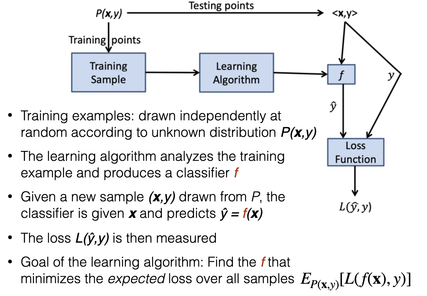
By training dataset, we get a model h for mapping input to output. The overall goal of surpvised learning is to find the model h that approximate function f that maps x to y, i.e. f(x) = y. The closer that h to f, the better the model is. Model is not a mysterious blackbox, instead, it’s just a mathematical representation of a system used to make predictions. The model can range from a simple linear mapping to a highly complex one.

The hypothesis is used to guide the learning process of the model, it’s a decision or assumption made by ourself. For example, for a price prediction problem, my hypthesis could be defined as linear regression models. So I will say the price prediction equation is h(x) = w0 + w1 * quantity + w2 * quality_score + w3 * location. This equation describes all the possible hypothesis for this problem, i.e. hypothesis space. Each hypothesis is represented as h that has specified values of weights. However, hypothesis does have limitations. What if the pricing problem cannot be predicted by linear regression? What if we need a more complex model? In this case, we need to modify the hypothesis to expand the hypothesis space.

Training Process and Prediction

What is the process of model training?

Just like us, learning is a tough process for machine as well. Learning takes thousands and millions rounds of failure and improvements. Here are the general steps of training process:

Steps of model training:

1. Data preparation: prepare the training and testing dataset discussed above.

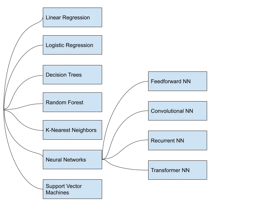
2. Model selection/Learning algorithm: select appropriate algorithm for specific problem

   In supervised learning, the most common types of learning algorithms are summarized below: (of course, there’re more algorithms)

   

3. Model Training: using training dataset to train the model and obtain the optimal parameters.

4. Validation via Loss Function (Objective Function): using the testing dataset to evaluate the performance of the model.

5. Fine-tuning: based on the performance of the model on the testing dataset, training will adjust the parameters for higher accuracy.

Loss function and Objective function

What is loss function?

What are the differences between loss function and objective function?

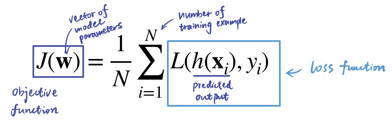
By definition, a loss function measures the difference between the predicted output of a machine learning model and the actual output. It measures how well the model predicts the output given a set of input x.

On the other hand, Objective function measures the accuracy of the model’s predictions against the true output values in the training data. Objective function measures the overall model accuracy. Objective function takes sum all loss functions and average it by the number of training samples.

Equation of Objective function and the meaning of each part:

Classification vs. Regression

Classification and regression describe two types of supervised learning model based on the model utility. In short:

• Classification is used when target variable is categorical.
  • E.g. Classify this object as either a balloon or not.
• Regression is used when target variable is continuous.
  • E.g. The target variable is the price and we want to predict it.

Model Fitting

Overfitting vs. underfitting

These are the two most common issues for a machine learning model.

• Overfitting occurs if a model is trained too closely on the training set. So that the model doesn’t perform well on new data, e.g. testing set. We describe the model as not generalize well in this case.
• Underfitting means a model is too simple and cannot capture the mapping between input and output, i.e perform poorly on both testing and training set.

Variance vs. bias trade-off

• Variance refers to the amount by which the predicted outcomes of a model vary for different training datasets.
• Bias is the difference between the average prediction of our model and the correct value which we are trying to predict.

If a model is too complex, then the model is likely to be overfitting. In this case, the model has a high variance and low bia. Because the model predicts the training set accurately but does not generalize well on new data.

Linear threshold units (LTUs) and Perceptron

Linear threshold units

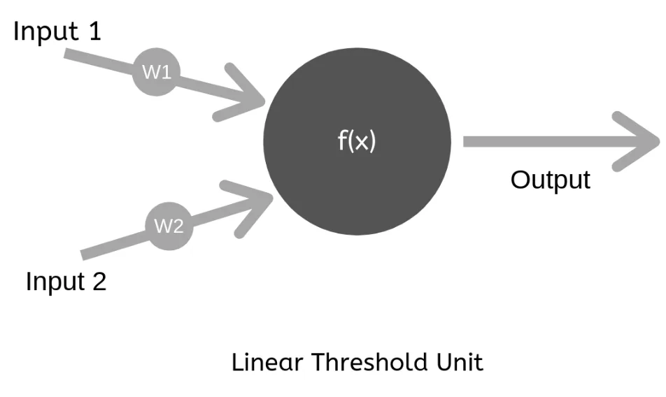
This is the very first linear model used in surpervised learning. The reason we call it “linear” is because LTU performs a linear combination of inputs x and weights w. The reason behind “threshold” is that LTU uses step activation function, i.e. if reaches threshold predicted value h(x) = 1, otherwise h(x) = 0.

LTU equation: w is a vector of weights, x is input, b is bias.

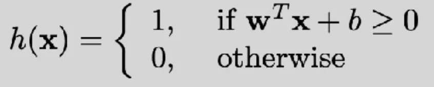
Combining with the hypothesis space concept we learned above, we find that the hypothesis space of LTU is Fixed Size, Deterministic, and has Continuous parameters. Also, it’s worth to note that Linear threshold units can only be used for binary classification.

LTU Graphical Representation: Source

Perceptron

Perceptron is simply one or multiple LTUs in one layer. Each LTU can be used for binary classification. By having multiple LTUs in one layer, i.e. perceptron, we can perform multi-class classification. The Loss function used by perceptron is hinge-loss function, so that gradient descent optimization is feasible.

Perceptron linear model has a relatively simple implementation, thus faster training speed and better intepretability. However, since perceptron is a linear model, so the data must be linearly separable. Perceptron may also overfit if there’re too many input features. For non-linearly separable data, we need to use non-linear model, such as multi-layer perceptron and decision tree.

Logistic Regression

Unlike perceptron learns the direct mapping y = f(x), logistic regression learns the conditional probability P(y|x), i.e. given x, what is the probability of y (Learning a distribution). The learning goal is to find the most likely distribution given the training data.

Sigmoid Activation Function

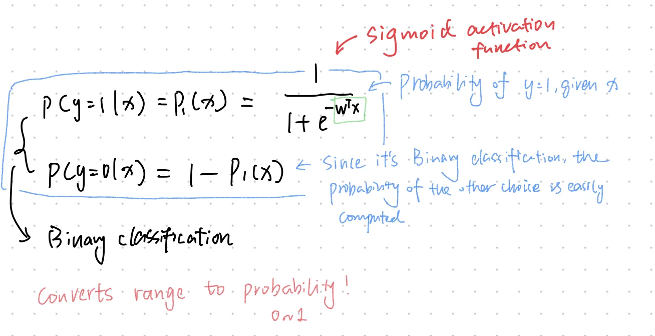
Logistic regression uses sigmoid activation function to map the dependent variable y_hat into values between 0 and 1, so that this value can be interpreted as probability. Also note that each feature must be independent in logistic regression model.

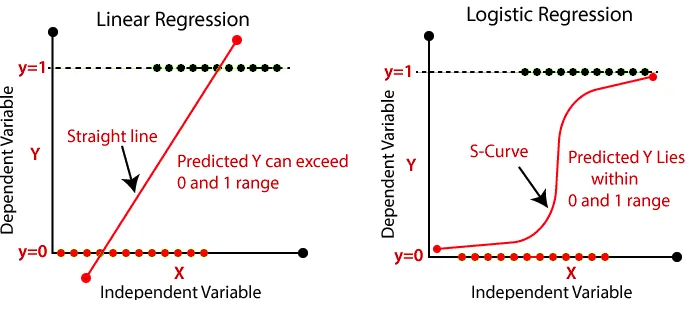
The conditional probability in mathematical formula is:Sigmoid function ranges from 0 to 1, and it introduces non-linearity to model. Also, exp is differentiable and easy to learn, which also handles noisy labels naturally.

Cross Entropy Loss

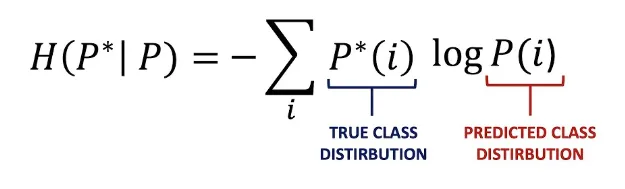
Logistic regression model uses cross entropy loss function to measure the accuracy of model. Cross entropy measures the difference between predicted distribution and actual distribution.

Softmax Activation Function

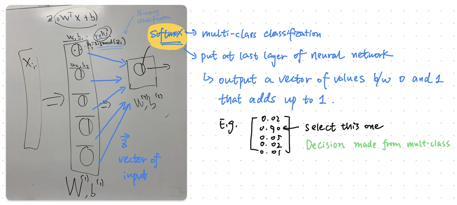
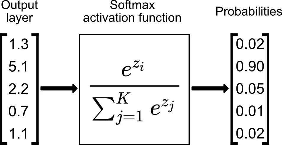
Logistic regression outputs the probabilty of input a belongs to certain class, which is a binary classifcation. But what if we want to use multi-class classification? In this case, you need to use softmax activation function at the output layer of neural network.

Neural network implementation

Softmax function

Overall, logistic regression is relatively easy to implement and highly interpretable. But logistic regression is sensitive to outliers and requires features to be independent.

Linear Discrimination Analysis

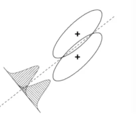
The goal of LDA is to learn the joint distribution p(x, y) between input features and output. It’s a statistical technique used to find a linear combination of features that best separates or discriminates between two or more classes. The separation is illustrated by the graph below.

Two classes of data are separated by a line

Unlike other linear model, LDA has a strong assumption to data, which is: Data are normally distributed, or in another word, following the Gaussian distribution. Also, the classes defined must have same covariance matrix.

Linear discrimination analysis will calculate and give a Linear discriminant function that separates classes. That means LDA does not need training, instead LDA is just calculations. This function is derived using class means and covariances of input variables. The goal of this function is to maximize the ratio of the between-class variance to the within-class variance, so that classes are separated in the best possible way. There’re two rules of classification that LDA can use, one is Bayes discriminant rule and the other is Maximum likelihood rule. You can view LDA as computing Mahalanobis Distance for all classes and then classifying x according to which mean it’s closest to.

LDA is a generative model because it can generate new data based on the model. On the other hand, logistic regression and perceptron are predictive models because they can only make predictions. If the generative model is correct, LDA gives highest accuracy. It also requires less data to get the model compared to other models like logistic regression. Meanwhile, LDA is robust to missing values and noise. However, LDA has strong model assumption, i.e. data must be normally distributed. If the assumption is violated, model will perform poorly.

Model Optimization: Gradient Descent Algorithm

The reason we use gradient descent is to find the optimal parameters of model. There are three types of Gradient descent algorithms: Batch GD, mini-Batch GD, and Stochastic GD.

Batch gradient descent works on the entire training dataset, while stochastic gradient descent works on one random sample at a time, and mini-batch gradient descent works on a group of sample each time.

Thus batch gradient descent requires a large amount of computational resources. Meanwhile, Batch gradient descent converges more smoothly but more slowly compared to the other two. The convergence curves are compared below.

Convergence cureve between GD and Stochastic GD

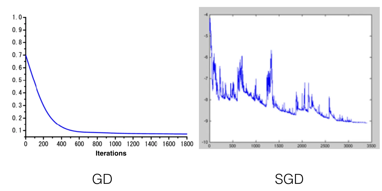
Stochastic GD and mini-batch GD have better generalization compared to batch GD. However, they are more likely to introduce noise during convergence. Overall, there are pros and cons to these three gradient descent methods, and we must make trade-offs when making decisions.

Keep Learning! : )